Kyung D. kim

• Back

Cyclistic Analysis
__
About the company
In 2016, Cyclistic launched a successful bike-share offering. Since then, the program has grown to a fleet of 5,824 bicycles that are geotracked and locked into a network of 692 stations across Chicago. The bikes can be unlocked from one station and returned to any other station in the system anytime.Objective: Design marketing strategies aimed at converting casual riders into annual members.Ask
In this project, I will conduct an extensive analysis of the 2019 datasets spanning quarters 1 through 4. This thorough examination aims to provide a comprehensive understanding of the usage patterns between casual and annual members throughout the year. By addressing key questions such as differential usage behaviors and motivations behind casual riders and annual memberships, I aim to uncover actionable insights.The data analysis will unveil an opportunity to attract a new segment of annual members by encouraging casual weekend riders to switch to annual memberships. Furthermore, by strategically targeting marketing efforts around stations with the highest usage, Cyclistic can maximize their outreach.To incentivize conversions, the marketing team can implement initiatives such as offering prizes or discount opportunities to riders who share their experiences on social media platforms. This approach not only encourages increased ridership but also promotes the value proposition of annual memberships, ultimately driving higher conversion rates.Prepare
Downloaded 2019 Q1 to Q4 files from
https://divvy-tripdata.s3.amazonaws.com/index.htmlDivvyTrips2019Q1
DivvyTrips2019Q2
DivvyTrips2019Q3
DivvyTrips2019Q4
Imported files to SQL Server Management Studio (SSMS)Prepare the tables to create one larger table.
Renamed column names to be consistent across all four tables.
sql
exec sp_rename 'dbo.Divvy_Trips_2019_Q2._01_Rental_Details_Rental_ID','trip_id';
exec sp_rename 'dbo.Divvy_Trips_2019_Q2._01_Rental_Details_Local_Start_Time','start_time';
exec sp_rename 'dbo.Divvy_Trips_2019_Q2._01_Rental_Details_Local_End_Time','end_time';
exec sp_rename 'dbo.Divvy_Trips_2019_Q2._01_Rental_Details_Bike_ID','bikeid';
exec sp_rename 'dbo.Divvy_Trips_2019_Q2._01_Rental_Details_Duration_In_Seconds_Uncapped','tripduration';
exec sp_rename 'dbo.Divvy_Trips_2019_Q2._03_Rental_Start_Station_ID','from_station_id';
exec sp_rename 'dbo.Divvy_Trips_2019_Q2._03_Rental_Start_Station_Name','from_station_name';
exec sp_rename 'dbo.Divvy_Trips_2019_Q2._02_Rental_End_Station_ID','to_station_id';
exec sp_rename 'dbo.Divvy_Trips_2019_Q2._02_Rental_End_Station_Name','to_station_name';
exec sp_rename 'dbo.Divvy_Trips_2019_Q2.User_Type','usertype';
exec sp_rename 'dbo.Divvy_Trips_2019_Q2.Member_Gender','gender';
exec sp_rename 'dbo.Divvy_Trips_2019_Q2._05_Member_Details_Member_Birthday_Year','birthyear';

Renamed table names to simplify when referencing
sql
exec sp_rename 'dbo.Divvy_Trips_2019_Q1','trips2019Q1';
exec sp_rename 'dbo.Divvy_Trips_2019_Q2','trips2019Q2';
exec sp_rename 'dbo.Divvy_Trips_2019_Q3','trips2019Q3';
exec sp_rename 'dbo.Divvy_Trips_2019_Q4','trips2019Q4';

Modified the records under usertype to be clearer and consistent.
sql
update trips2019Q1
set user_type = 'member'
where user_type = 'subscriber';
update trips2019Q1
set user_type = 'casual'
where user_type = 'customer';
update trips2019Q2
set user_type = 'member'
where user_type = 'subscriber';
update trips2019Q2
set user_type = 'casual'
where user_type = 'customer';
update trips2019Q3
set user_type = 'member'
where user_type = 'subscriber';
update trips2019Q3
set user_type = 'casual'
where user_type = 'customer';
update trips2019Q4
set user_type = 'member'
where user_type = 'subscriber';
update trips2019Q4
set user_type = 'casual'
where user_type = 'customer';

Added a column for day number of the week and a column for day of the week.
Then created a view of all 4 quarters combined.
sql
create view [dbo].[v_FY2019] as
SELECT [trip_id]
,[start_time]
,[end_time]
,[bikeid]
,[tripduration]
,[from_station_id]
,[from_station_name]
,[to_station_id]
,[to_station_name]
,[usertype]
,[gender]
,DATEPART(WEEKDAY,start_time) as day_number
,DATENAME(dw,start_time) as day_of_week
FROM [Cyclistic].[dbo].[trips2019Q1]
Union all
SELECT [trip_id]
,[start_time]
,[end_time]
,[bikeid]
,[tripduration]
,[from_station_id]
,[from_station_name]
,[to_station_id]
,[to_station_name]
,[usertype]
,[gender]
,DATEPART(WEEKDAY,start_time) as day_number
,DATENAME(dw,start_time) as day_of_week
FROM [Cyclistic].[dbo].[trips2019Q2]
union all
SELECT [trip_id]
,[start_time]
,[end_time]
,[bikeid]
,[tripduration]
,[from_station_id]
,[from_station_name]
,[to_station_id]
,[to_station_name]
,[usertype]
,[gender]
,DATEPART(WEEKDAY,start_time) as day_number
,DATENAME(dw,start_time) as day_of_week
FROM [Cyclistic].[dbo].[trips2019Q3]
union all
SELECT [trip_id]
,[start_time]
,[end_time]
,[bikeid]
,[tripduration]
,[from_station_id]
,[from_station_name]
,[to_station_id]
,[to_station_name]
,[usertype]
,[gender]
,DATEPART(WEEKDAY,start_time) as day_number
,DATENAME(dw,start_time) as day_of_week
FROM [Cyclistic].[dbo].[trips2019Q4]
GO

Process
– Year column was not included in the view, because it does not seem accurate. Some rows had 1900 as the year.Checked min and max of the start_time to make sure it is only for 2019
sql
select min(start_time)
,max(start_time)
from v_FY2019;

Analyze
Made some initial measurements and explored the data.
sql
create view [dbo].[v_FY2019_measurements] as
--use Cyclistic
--go
select usertype
, CONCAT('QTR ',DATEPART(quarter,start_time)) as qtrly
, day_number
, day_of_week
, AVG(tripduration) as avg_ride_duration
, SUM(tripduration) as Ttl_duration_time
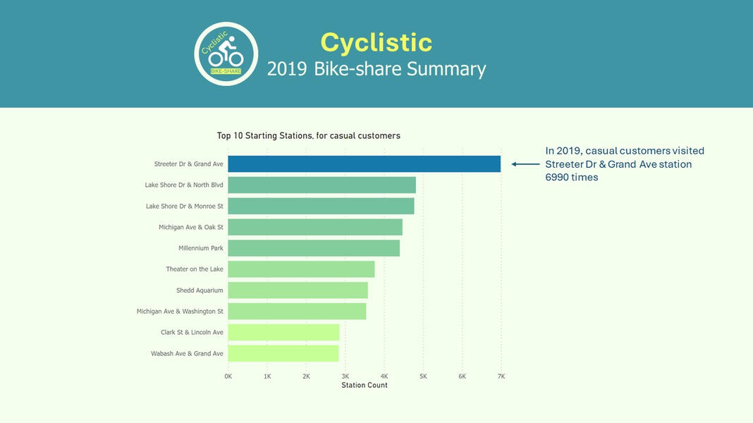
, from_station_name
, count(from_station_name) as from_station_count
, to_station_name
, COUNT(to_station_name) as tp_station_count
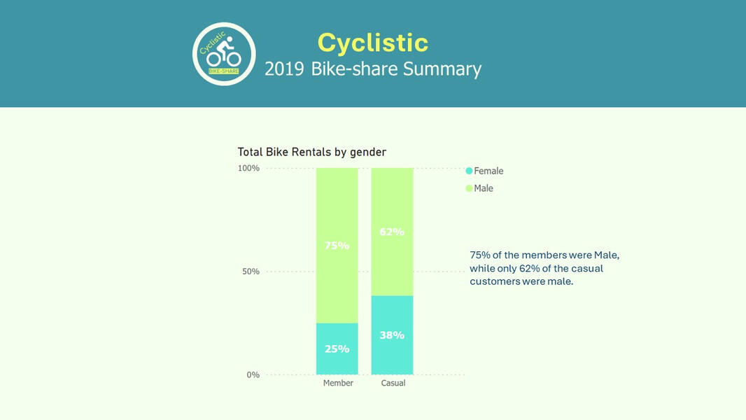
, gender
, COUNT(trip_id) as total_ride
from v_fy2019
group by usertype,
DATEPART(quarter,start_time)
, day_number
, day_of_week
, from_station_name
, to_station_name
, gender
GO

From here, I imported the data into Power BI to visualize and run further analysis, which can be seen in the PowerPoint Presentation section.

• Back

R
getinstall.packages("tidyverse")# Set working directory and check
setwd("/Users/KD3/Documents/Data Analysis/cyclisticgoogle coursera project/database")getwd()# Install packages needed to. Data wrangling and visualization packages
library(tidyverse)
library(lubridate)
library(ggplot2)# Import datasets (csv)
Trips2019Q1 <- read.csv("DivvyTrips2019Q1.csv")
Trips2019Q2 <- read.csv("DivvyTrips2019Q2.csv")
Trips2019Q3 <- read.csv("DivvyTrips2019Q3.csv")
Trips2019Q4 <- read.csv("DivvyTrips2019Q4.csv")
Trips2020Q1 <- read.csv("DivvyTrips2020Q1.csv")WRANGLE DATA AND COMBINE INTO A SINGLE FILE# Columns were renamed, using the 2020Q1 column names, for consistency. But also it is the latest dataset, which assumes the column names will be this going forward.(Trips2019Q1 <- rename(Trips2019Q1
,rideid = tripid
,rideabletype = bikeid
,startedat = starttime
,endedat = endtime
,startstationname = fromstationname
,startstationid = fromstationid
,endstationname = tostationname
,endstationid = tostationid
,membercasual = usertype))(Trips2019Q3 <- rename(Trips2019Q3
,rideid = tripid
,rideabletype = bikeid
,startedat = starttime
,endedat = endtime
,startstationname = fromstationname
,startstationid = fromstationid
,endstationname = tostationname
,endstationid = tostationid
,membercasual = usertype))(Trips2019Q4 <- rename(Trips2019Q4
,rideid = tripid
,rideabletype = bikeid
,startedat = starttime
,endedat = endtime
,startstationname = fromstationname
,startstationid = fromstationid
,endstationname = tostationname
,endstationid = tostationid
,membercasual = usertype))(Trips2019Q2 <- rename(Trips2019Q2
,rideid = X01...Rental.Details.Rental.ID
,rideabletype = X01...Rental.Details.Bike.ID
,startedat = X01...Rental.Details.Local.Start.Time
,endedat = X01...Rental.Details.Local.End.Time
,startstationname = X03...Rental.Start.Station.Name
,startstationid = X03...Rental.Start.Station.ID
,endstationname = X03...Rental.Start.Station.Name
,endstationid = X02...Rental.End.Station.ID
,membercasual = User.Type))# Inspect the dataframes and look for inconguenciesstr(Trips2019Q1)
str(Trips2019Q2)
str(Trips2019Q3)
str(Trips2019Q4)
str(Trips2020Q1)# Rideid and rideabletype changed to character in 2020 Q1#Convert rideid and rideabletype to character so that they can stack correctly.Trips2019Q1 <- mutate(Trips2019Q1, rideid = as.character(rideid)
,rideabletype = as.character(rideabletype))
Trips2019Q2 <- mutate(Trips2019Q2, rideid = as.character(rideid)
,rideabletype = as.character(rideabletype))
Trips2019Q3 <- mutate(Trips2019Q3, rideid = as.character(rideid)
,rideabletype = as.character(rideabletype))
Trips2019Q4 <- mutate(Trips2019Q4, rideid = as.character(rideid)
,rideabletype = as.character(rideabletype))# Stack individual quarter's data frames into one big data frame
alltrips <- bindrows(Trips2019Q1,Trips2019Q2,Trips2019Q3,Trips2019Q4,Trips2020Q1)# Remove lat, long, birthyear, and gender fields as this data was dropped beginning in 2020
alltrips <- alltrips %>%
select(-c(endlng,endlat,startlng,startlat,"X05...Member.Details.Member.Birthday.Year","Member.Gender",birthyear,tripduration,"X02...Rental.End.Station.Name","X01...Rental.Details.Duration.In.Seconds.Uncapped",gender))CLEAN UP AND ADD DATA TO PREPARE FOR ANALYSIS# Inspect the new table
colnames(alltrips)
9 columnsnrow(alltrips)
4244891dim(alltrips)
head(alltrips)
tail(alltrips)
str(alltrips)
summary(alltrips)unique(alltrips$membercasual)
[1] "Subscriber" "Customer" "member" "casual"# “member casual” column has 4 unique names. Need to consolidate them to just member or customertable(alltrips$membercasual)# Reassign to desired values, using the 2020 labels.alltrips <- alltrips %>%
mutate(membercasual = recode(membercasual
,"Subscriber" = "member"
,"Customer" = "casual"))# Check to make sure the proper number of observations were reassigned
table(alltrips$membercasual)
casual member
929117 3315774# Add a date column, month,day, and year of each ride.
alltrips$date <- as.Date(alltrips$startedat)
alltrips$month <- format(as.Date(alltrips$date), "%m")
alltrips$day <- format(as.Date(alltrips$date), "%d")
alltrips$year <- format(as.Date(alltrips$date), "%Y")
alltrips$dayofweek <- format(as.Date(alltrips$date), "%A")# Add a "ridelength" calculation to alltrips (in seconds)
alltrips$ridelength <- difftime(alltrips$endedat,alltrips$startedat)# Convert "ridelength" from Factor to numeric so we can run calculations on the data
alltrips$ridelength <- as.numeric(as.character(alltrips$ridelength))
#check
is.numeric(alltrips$ridelength)# Remove bad data. Remove negative ridelength
# Create a new version alltripsv2 since data is being removed
alltripsv2 <- alltrips[!(alltrips$ridelength<0),]CONDUCT DESCRIPTIVE ANALYSIS# Descriptive analysis on ridelength (all figures in seconds)
summary(alltripsv2)
mean(alltripsv2$ridelength)
1438.08
median(alltripsv2$ridelength)
691
max(alltripsv2$ridelength)
10628422
min(alltripsv2$ridelength)
0# I do have concern that some of the ridelength that are roughly under a minute* may skew the aggregate measurements of ride time for customers actually using them. Those seem more like testing or errors because renting and riding a bike for under a minute seems odd. They are kept because I don’t have the answer.
# This could be good data to track how many are under a minute or so to see why that is happening.
# Are people struggling with the rental process?
# Were these mistakes?
# Was it to test how the rental bikes worked?# Compare members and casual users
aggregate(alltripsv2$ridelength ~ alltripsv2$membercasual, FUN = mean)
1 casual 3542.9107
2 member 848.3597aggregate(alltripsv2$ridelength ~ alltripsv2$membercasual, FUN = median)
1 casual 1537
2 member 579aggregate(alltripsv2$ridelength ~ alltripsv2$membercasual, FUN = max)
1 casual 10628422
2 member 9056634aggregate(alltripsv2$ridelength ~ alltripsv2$membercasual, FUN = min)
1 casual 0
2 member 1# See the average ride time by each day for members vs casual users
aggregate(alltripsv2$ridelength ~ alltripsv2$membercasual + alltripsv2$dayofweek, FUN = mean)
1 casual Friday 3753.8207
2 member Friday 825.5616
3 casual Monday 3323.7529
4 member Monday 845.8592
5 casual Saturday 3339.8682
6 member Saturday 973.6027
7 casual Sunday 3559.3345
8 member Sunday 927.2223
9 casual Thursday 3780.3311
10 member Thursday 811.8656
11 casual Tuesday 3536.6105
12 member Tuesday 829.8384
13 casual Wednesday 3676.3186
14 member Wednesday 813.8006# The days of the week are out of order.
alltripsv2$dayofweek <- ordered(alltripsv2$dayofweek, levels=c("Sunday", "Monday", "Tuesday", "Wednesday", "Thursday", "Friday", "Saturday"))# Average ride time by each day for members vs casual users
aggregate(alltripsv2$ridelength ~ alltripsv2$membercasual + alltripsv2$dayofweek, FUN = mean)
1 casual Sunday 3559.3345
2 member Sunday 927.2223
3 casual Monday 3323.7529
4 member Monday 845.8592
5 casual Tuesday 3536.6105
6 member Tuesday 829.8384
7 casual Wednesday 3676.3186
8 member Wednesday 813.8006
9 casual Thursday 3780.3311
10 member Thursday 811.8656
11 casual Friday 3753.8207
12 member Friday 825.5616
13 casual Saturday 3339.8682
14 member Saturday 973.6027# Analyze ridership data by type and weekday
alltripsv2 %>%
mutate(weekday = wday(startedat, label = TRUE)) %>%
groupby(membercasual, weekday) %>%
summarise(numberofrides = n()
,averageduration = mean(ridelength)) %>%
arrange(membercasual, weekday)
membercasual weekday numberofrides averageduration
<chr> <ord> <int> <dbl>
1 casual Sun 185059 3559.
2 casual Mon 106324 3324.
3 casual Tue 93912 3537.
4 casual Wed 95639 3676.
5 casual Thu 106236 3780.
6 casual Fri 126288 3754.
7 casual Sat 215536 3340.
8 member Sun 292198 927.
9 member Mon 520703 846.
10 member Tue 566722 830.
11 member Wed 558255 814.
12 member Thu 548160 812.
13 member Fri 512462 826.
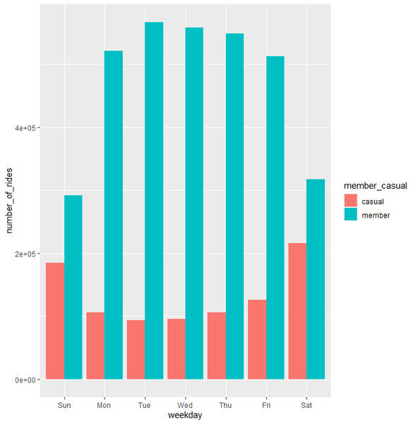
14 member Sat 317267 974.# Visualize the number of rides by rider type
alltripsv2 %>%
mutate(weekday = wday(startedat, label = TRUE)) %>%
groupby(membercasual, weekday) %>%
summarise(numberofrides = n()
,averageduration = mean(ridelength)) %>%
arrange(membercasual, weekday) %>%
ggplot(aes(x = weekday, y = numberofrides, fill = membercasual)) +
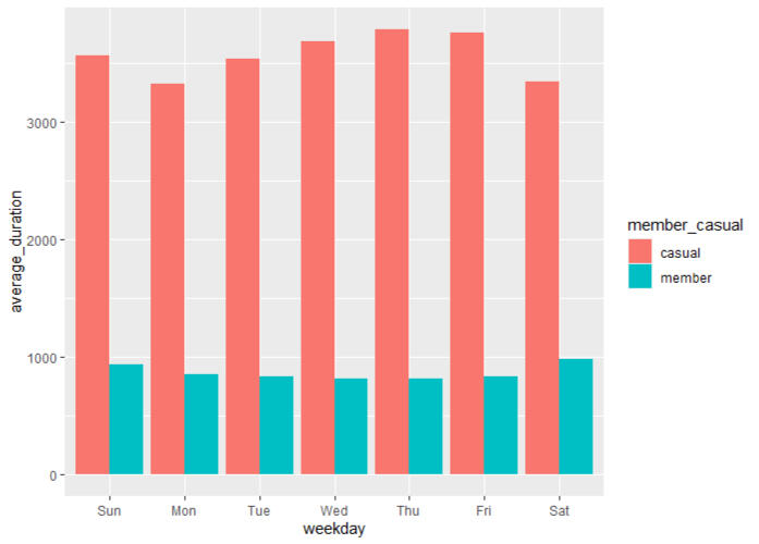
geomcol(position = "dodge")# Create a visualization for average duration
alltripsv2 %>%
mutate(weekday = wday(startedat, label = TRUE)) %>%
groupby(membercasual, weekday) %>%
summarise(numberofrides = n()
,averageduration = mean(ridelength)) %>%
arrange(membercasual, weekday) %>%
ggplot(aes(x = weekday, y = averageduration, fill = membercasual)) +
geomcol(position = "dodge")# Export csv file for further visualization, Power BI
write.csv(alltripsv2, "C:\Users\KD3\Documents\Data Analysis\cyclisticgoogle coursera project\database\alltripsv2.csv", row.names=FALSE)

• Back

How to buy a new car

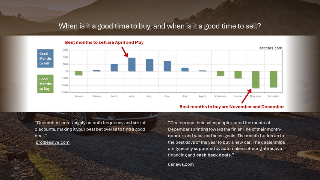
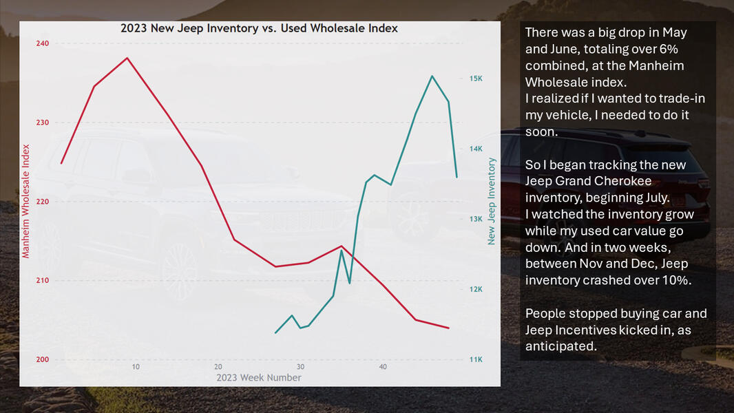
Jeep New Car Inventory was compiled by tracking nationwide availability weekly for six months on cars.com.Other resources include:
- iseecars.com
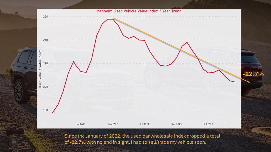
- Manheim used Wholesale Index
- edmunds.com